

Map Description and Instructions
This web map application for the NRCS-funded Sage Grouse Initiative visualizes, distributes, and interactively analyzes spatial data produced by the SGI’s science team. We have provided descriptions and instructions below for how to use and download this sagebrush-steppe data.
- Tree Canopy Cover data description
- Ecosystem Resistance & Resilience data description
- Cultivation Risk data description
- Fence Collision data description
- Instructions to view in ArcGIS
- Instructions to view in QGIS
- Instructions for bulk download
Data Descriptions
Tree Canopy Cover
This product provides a high-resolution estimate of tree canopy cover on a per-acre basis. Thematic raster data represents tree canopy cover (% cover per acre) in the following classes:
- less than 1% or absent
- 1 – 4%
- 4 – 10%
- 10 – 20%
- 20 – 50%
- greater than 50%
Data are in 1 meter spatial resolution suitable for analysis in a GIS. The canopy cover product is derived from 1 meter 4-band NAIP imagery from various years (see below). A spatial wavelet analysis (SWA) algorithm was implemented in MATLAB for conifer detection. It is intended to target conifer canopy cover; however, the SWA method used detects non-conifer tree species in some situations. Therefore, users should ground truth results when making site-specific land management decisions. SWA is particularly good at detecting conifer trees in arid environments, although has known limitations. The SWA algorithm requires a minimum of 2-3 pixels in width for tree detection. Therefore, the minimum tree detection size using 1m spatial resolution NAIP imagery is 2-3m in diameter. Conifer tree detection accuracy decreases in mesic environments such as wetlands, riparian areas and mountainous zones where mixed deciduous and conifer tree diversity exists. This map provides an estimate of conifer cover on a per-acre basis based on a census of all trees, not exclusively encroaching trees.
| State | NAIP Year |
| California | 2012 |
| Colorado | 2013 |
| Idaho | 2013 |
| Montana | 2013 |
| Nevada | 2013 |
| Oregon | 2012 |
| Utah | 2011 |
* Produced by Michael Falkowski, Nilam Kayastha, and Aaron J. Poznanovic
Ecosystem Resistance & Resilience
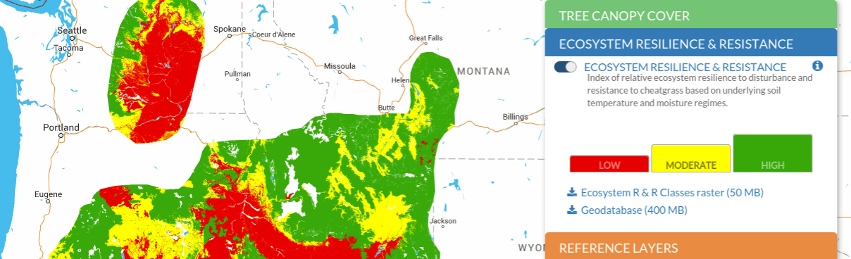
This layer depicts a simplified index of relative ecosystem resilience to disturbance and resistance to cheatgrass (“R&R”), providing a tool for rapid risk assessment across sage-grouse habitats in the western range. Potential ecosystem R&R depends in part on the biophysical conditions an area is capable of supporting and soil temperature and moisture regimes can be used to depict this gradient at large scales (Chambers et al. 2014). Soils data were derived from two primary sources: 1) completed and interim soil surveys available through the Soil Survey Geographic Database (SSURGO), and 2) the State Soils Geographic Database (STATSGO2) to fill gaps where SSURGO data were not available. Using best available information and expert input, each soil temperature and moisture regime/moisture subclass was placed into one of three categories of relative R&R: high, moderate, and low (Table 1; Maestas et al. 2016). Soils with high water tables, wetlands, or frequent ponding that would not typically support sagebrush were not rated.
This tool is most appropriate for regional and landscape level planning and prioritization. When combined with other data layers, such as the sage-grouse PACs and existing land cover, planners can use this tool to inform where to prioritize strategic actions before, during, and after wildfire to conserve sagebrush habitats and prevent conversion to annual grasslands. At more local scales, depicting the actual soil temperature/moisture subclasses included in the file geodatabase, rather than just the index, provides a more nuanced view of the environmental gradient. Application of this tool is just one step in the planning process and must be followed by more detailed site assessments to verify soils and incorporate additional factors, such as current vegetation condition, that heavily influence R&R.
Table 1. Rating of relative resilience and resistance across predominant rangeland ecosystems in the western sage-grouse range. From Maestas et al. 2016.
|
Soil Temperature and Moisture Regime, Moisture Subclass |
Common Name |
Typical Shrub Type |
R&R Rating |
|
Cryic/Xeric-Typic |
Cold/moist |
Mountain big sagebrush, mountain brush |
High |
|
Cryic/Xeric bordering on Aridic |
Cold/moist bordering on dry |
Mountain big sagebrush |
High |
|
Frigid/Xeric-Typic |
Cool/moist |
Mountain big sagebrush, mountain brush |
High |
|
Cryic/Aridic bordering on Xeric |
Cold/dry bordering on moist |
Mountain big sagebrush, low sagebrush |
High |
|
Cryic/Aridic-Typic |
Cold/dry |
Low sagebrush |
Moderate |
|
Frigid/Xeric bordering on Aridic |
Cool/moist bordering on dry |
Mountain big sagebrush |
Moderate |
|
Frigid/Aridic-Typic |
Cool/dry |
Mountain/Wyoming big sagebrush, low sagebrush |
Moderate |
|
Frigid/Aridic bordering on Xeric |
Cool/dry bordering on moist |
Mountain/Wyoming big sagebrush, low sagebrush |
Moderate |
|
Mesic/Xeric-Typic |
Warm/moist |
Wyoming big sagebrush, basin big sagebrush |
Moderate |
|
Mesic/Xeric bordering on Aridic |
Warm/moist bordering on dry |
Wyoming big sagebrush, black sagebrush |
Low |
|
Mesic/Aridic bordering on Xeric |
Warm/dry bordering on moist |
Wyoming big sagebrush, basin big sagebrush |
Low |
|
Mesic/Aridic-Typic |
Warm/dry |
Salt desert shrub |
Low |
Maestas et al. 2016. Tapping Soil Survey Information for Rapid Assessment of Sagebrush Ecosystem Resilience and Resistance. Rangelands.
Chambers et al. 2014. Using resistance and resilience concepts to reduce impacts of annual grasses and altered fire regimes on the sagebrush ecosystem and sage-grouse– A strategic multi-scale approach. Fort Collins, CO, USA: U.S. Department of Agriculture, Forest Service, RMRS-GTR-326.
Maestas, J. D., and S. B. Campbell. 2014. Mapping Potential Ecosystem Resilience and Resistance across Sage-Grouse Range using Soil Temperature and Moisture Regimes. Fact Sheet. Sage Grouse Initiative.
Cultivation Risk
This product represents the probability of cultivation relative to climate (30 year normalization of mean annual precipitation, mean annual temperature, number of degree days greater than five degrees C, and duration of frost free period); soils (water holding capacity and other hydrological characteristics); and topography (compound topographic index, neighborhood roughness, slope, and surface relief).
Various dataets were used, including regional climate data, USDA NRCS SSURGO, and USDA NASS Cropland Data Layer (CDL). Independent models were produced for each county; county level predicitons were merged for state coverage.
Data are available by state:
Produced by Jeff Evans, The Nature Conservancy.
Smith, J.T., J.S. Evans, B.H. Martin, S. Baruch-Mordo, J.M. Kiesecker, and D.E. Naugle. In review. Reducing cropland conversion risk to sage-grouse through strategic conservation of working rangelands.
Fence Collision
The fence collision tool visualizes and exports sage grouse fence collision risk relative to lek locations or other areas of high bird concentration. It is based on models described in Stevens et al. (2013). This service is in Beta and is not guaranteed. If visualization fails, export will likely continue to function.
After toggling the layer on, use the drawing tools  in the upper left hand corner to place points or draw polygons. Points represent lek locations; fence collision risk is calculated relative to distance from the lek, up to a maximum three km. Polygons represent areas of bird concentration, e.g., wintering grounds. Fence collision risk is calculated the same as points, except that distance is removed; everything within the polygon is treated as a distance of zero.
Alternatively, a zipped shapefile of points or polygons can be uploaded. The zipped file must contain the .shp, .prj, and .shx files of the shapefile, and must only contain 2D geometries. Commonly used coordinate reference systems and projections are supported. Attributes are ignored. An example of a zipped shapefile is available. Once submitted, the points or polygons of the shapefile will be displayed on the map; additional points or polygons can be added using the drawing tools. Please note that there may be a lag while processing the shapefile; processing was optimized for individual states. If necessary, follow these instructions to convert 3D shapefiles to 2D shapefiles using ESRI ArcMap.
Click ‘Calculate layer’ to visualize fence collision risk. Click ‘Reset layer’ to reset point and polygon features. The visualization is scale dependent. For more accurate results it is necessary to zoom to an appropriate level. When fence collision risk is visualized, the data may be exported as a raster GeoTiff. This allows the data to be brought into GIS software and used for planning purposes within other projects. Enter your email address in the box and click ‘Download layer’. A confirmation will appear and the recipient will be notified via email when the layer is ready. Downloads are available for five days. Large areas will be exported as multiple files and may be subsequently merged into one file within GIS software.
Lek information is temporarily cached for processing; it is automatically deleted after one day. Lek information is not archived or permanently stored. All lek information is transported securely.
Stevens, B. S., D. E. Naugle, B. Dennis, J. W. Connelly, T. Griffiths, and K. P. Reese. 2013. Mapping sage-grouse fence-collision risk: Spatially explicit models for targeting conservation implementation. Wildlife Society bulletin 37:409–415.
Instructions for Data Use and Download
To view in ArcGIS:
Data in the SGI web map application can be easily imported and viewed in ArcGIS without downloading big datasets. This allows for quick interaction with the data. For instance, users can add SGI data to a pre-existing project map or overlay other data on top of SGI data. These data can be imported as a web map tile service (WMTS) using the steps below.
The server URL: http://map.sagegrouseinitiative.com/wmts.xml
Connecting to WMTS
1. In the Catalog window, expand the GIS Servers node and double-click “Add WMTS Server”. Note: The images below reference WMS, but be sure to select WMTS.

- 2. Type in the server URL: http://map.sagegrouseinitiative.com/wmts.xml (You do not need to enter a user or password.)

- 3. Click “Get Layers” to see available layers.
- 4. Click “OK”.
To add the data to a the map:
Connect to a WMTS server in the Catalog window, choose “WMTS”, then drag it into your map.
OR
- Use the “Add Data” button.
- Click the “Add Data”
 button in the Standard toolbar to open the Add Data dialog box.
- Click the “Look” arrow and choose “GIS Servers”. This gives you a list of servers you have previously used. NOTE: If the server you want is not listed, you can connect to a WMTS server using the instructions above.
- After connecting to a WMTS server, the service is shown in the Add Data dialog box with this icon:

- Select this service.
- Click “Add”.
To View in QGIS:
Data in the SGI web map application can be easily imported and viewed in QGIS without downloading big datasets. This allows for quick interaction with the data, such as adding SGI data to a pre-existing project map or overlaying other data on top of this SGI data. These data can be imported as a web map tile service (WMTS) using the steps below:
The server URL: http://map.sagegrouseinitiative.com/wmts.xml
It may be necessary to first load an additional layer that overlaps the SGI data, e.g. a county polygon layer or project-specific layer.
- Under the Layer menu select “Add WMS/WMTS Layer”.
- Select “New” to add a service.
- Enter a name (use any name to identify SGI data, e.g. “SGI layers”) and the server URL: http://map.sagegrouseinitiative.com/wmts.xml
- Click “OK”.
- Click “Connect”.
- Select a layer and click “Add”.
- Click “Close”.
For bulk download:
Instructions coming soon.